Introduction
Download the file ex1.pde and run this program. For the rest of the exercises in this session, you only need to edit the "draw" method in the file.
Exercises
Exercise 1: drawing a line
The formula of a line between two points (x1,y1) en (x2,y2) is as follows:
(x-x1)*(y2-y1) = (y-y1)*(x2-x1)
1.1 Write a function
void drawLine(int x1, int y1, int x2, int y2)
that draws a straight line between the given coordinates. While processing already provides a built-in function (named line), the goal of this exercise is to learn how to write such a function yourself, given the more primitive function "point". Change the "draw" method such that a line is drawn rather than the random noise. Make sure your function works for lines in all 4 quadrants.
1.2 Which variable (x or y) did you use as the dependent and which as the independent variable? Why is the choice of dependent and independent variable important? How do you determine which variable to use as the independent one?
Exercise 2: fixed point arithmetic
On older machines, arithmetic with floating point numbers was a lot slower than arithmetic with integers. Therefore, most drawing routines where speed was of the essence (such as a line drawing algorithm) avoided using floating point numbers in their calculations.
2.1: in your algorithm of exercise 1, change all integers (int) to double-precision floating point numbers (double). What effect does this have?
Obviously, the algorithm no longer performs well because of rounding errors. The error can be illustrated by means of an example equation:
x = (y/6) * 8
Imagine both x and y are of type int. If y = 2, then x will be 0 (so the error = 2,66 - 0 = 2,66). One way to decrease this error (i.e. increase the precision) is to multiply both sides of the equation by a factor 10. This gives the result 10x = 10*(2/6)*8 = 24, so x is equal to 24/10 = 2. The error now is 2,66 - 2 = 0,66. By increasing the factor with which both sides are multiplied (e.g. 100), the precision of the result will increase even more.
The above method to work with floating point numbers solely by means of integer arithmetic is called fixed-point arithmetic. A regular floating point number (of type float or double) can be used to represent a very wide range of numbers using only a fixed bit size (32 resp. 64 bits). This is possible because the place of the decimal point (in dutch: de komma) in their representation can be at varying positions. If you only need a small range of values, you can represent a floating point number by an integer number by "fixing" the position of the decimal point.
Imagine you want to represent floating point numbers with a precision of 2 numbers after the decimal point. Also imagine that you only need to represent decimal numbers of at most 4 digits. With 4 digits, you can normally represent integers in the range 0 to 9999 (using decimal arithmetic). If you want a precision of 2 digits after the decimal point, then with the same amount of digits, you can represent 0,00 up to 99,99. This range of values is considerably less, but you can now represent fractional numbers!
The trick to fixed-point arithmetic is that we introduce an imaginary decimal point in the number, merely by programming convention (that is: by multiplying the number by 100 as in the first example). The computer does not know anything about this convention. For example, if we place the decimal point between digits 2 and 3 (as in the above example), then we represent the integer 5 by the actual integer 500 (because 500 = 0500 = 05,00 in our imaginary representation). A fractional number, such as 5,3 is represented by the actual integer 530 (because 530 = 0530 = 05,30). 21,65 is represented by the actual integer 2165, and so on. To turn an actual integer into a fixed-point integer, multiply by a "precision factor" (e.g. 100). To turn a fixed-point integer back into an actual integer, divide by the precision factor.
The fixed-point numbers that we have been using thus far are said to be formatted as '2:2', meaning 2 digits before and 2 digits after the decimal point. Up to now, we have been working with decimal digits (that can take on a value between 0 and 9). In computer science, we mostly work with binary digits (taking on a value of either 0 or 1). So a binary 16:16 fixed-point number is an integer of 32 bits, where the 16 most significant bits represent the integer part and the 16 least significant bits represent the fractional part of a number. Notice that, whereas a normal unsigned int can represent values in range [0,2^32 - 1], a 16:16 fixed-point unsigned int can only represent values in range [0,2^16 -1].
Doing arithmetic with fixed-point numbers has the advantage that the computer is manipulating integers while we interpret them as fractional numbers. Addition and subtraction are trivial in fixed-point arithmetic. For example, in decimal 2:2 format 5 + 4 is represented as 0500 + 0400 = 0900, and 0900 is interpreted as 9. This also works for fractional numbers: 22,15 - 1,4 is represented as 2215 - 0140 = 2075, and 2075 is interpreted as 20,75. This works as long as you interpret the result of an operation in the same fixed-point format as the input arguments.
Multiplication is less trivial. Consider 2,01 * 2,01. This is represented as 0201 * 0201 = 40401. While the two input arguments are 100x bigger than their interpretation, the output is 10.000x bigger (that is: 100a * 100b = 10.000ab). So either the output must be interpreted in the format 4:4 rather than 2:2 (i.e. 40401 = 00040401 ~ 0004,0401 = 4,0401) or you need to divide the result by 100 to convert it to 2:2 again (40401 / 100 = 404 = 0404 ~ 04,04). Note that because of this division, we lost 2 digits of precision (resulting in a rounding error of 0,0001).
When dividing two fixed-point numbers, the problem of multiplication does not appear. When dividing 100a / 100b, the factor 100 is cancelled out. However, 100a/100b = a/b, which is no longer a fixed-point number (you lose all precision)! For example 5,4 / 2 is represented as 0540 / 0200 = 2 (integer division). To interpret the result as a decimal 2:2 fixed-point number again, you need to multiply by 100 again (2*100 = 200 = 0200 ~ 02,00). Notice that 5,4 / 2 ought to be 2,7, so we lost our precision. To avoid this, rather than calculating (a/b)*100, it is better to calculate (a*100)/b: (0540 * 0100) / 0200 = 270 = 0270 ~ 02,70 = 2,7!
Notice that when multiplying or dividing fixed-point numbers, you have to be very careful for "overflows" in the intermediary results. If we only have 4 digits to store our decimal number, then we simply cannot store the intermediary number 40401 of the example multiplication. When multiplying two N:M fixed-point numbers, the result will have N+N:M+M digits. In the above examples, the results of multiplication and division were both 100x bigger than the representation of the input operands. When working with 32-bit numbers in a computer, be aware that fixed-point numbers which you multiply or divide can only have a maximum size of 16 bits. The first 16 bits can be divided into an integer and a fractional part, but the remaining 16 bits are required to store overflows.
2.2: apply fixed-point arithmetic to the formula of a line and integrate it in your algorithm. Turn the "precision" of your algorithm into a parameter. The other input parameters to the algorithm should remain unchanged and are still represented in integer screen coordinates.
2.3: in all of the above examples, I have been using decimal fixed-point numbers. Conversion between regular and fixed-point integers required multiplication or division by a certain decimal precision constant. There is, however, a more efficient way to do fixed-point arithmetic on a computer. When working with binary numbers, what precision factors would you choose? Why is this important? (hint: this factor is very easy to use when multiplying or dividing binary numbers).
Exercise 3: drawing a line using DDA
A downside of our line drawing algorithm is that it contains a lot of multiplications. On older computers, multiplication was a lot slower than addition or subtraction. We can remove some multiplications by taking the derivative of the equation of a line. For example, the derivative of 10x is 10.
So, instead of calculating the y-value at each x-coordinate that we plot between x1 and x2, we can also calculate it once at x1, and then just increase the y-value by 10 as we move towards x2. That is: for each increment in the x-value by 1, we increment the y-value by the differential. For lines, the differential is constant and is simply the slope (dutch: richtingscoefficient) of the line to plot. To see why this works, consider the equation yk = mxk + b with 0 < m <= 1. When increasing x by 1, we get:
              yk+1 = mxk+1 + b
              yk+1 = m(xk+1) + b
              yk+1 = mxk + m + b
              yk+1 = yk + m
Adapt your floating-point line drawing algorithm to use this technique, which is called a Digital Differential Analyzer.
Exercise 4: DDA + Fixed Point
Write a line algorithm using fixed-point arithmetic with 16 bits of precision and that uses DDA to save on the number of multiplications. Make sure it works in all 4 quadrants. This algorithm must not use floating point arithmetic.
Exercise 5: Bresenham's Algorithm
Bresenham's algorithm is a well-known line drawing algorithm and is very efficient as it only uses integer addition, bitshifts and equality tests involving 0. Given 2 points, Bresenham's algorithm draws a line by at each step making a choice between one of two pixels to plot. It chooses the pixel that is closest to the 'real line'.
Consider two points (x1,y1) and (x2, y2). Imagine (x1,y1) is the starting point. Given this pixel, there are 8 possible choices to plot the next pixel. It should be clear that only 2 of these 8 neighbouring points are relevant when drawing a line in the direction of (x2, y2). In what follows, consider 0 <= m <= 1 and x1 < x2 (in other words: the line is being drawn in the first octant). We consider x as the independent variable, which we increase by 1 at each step. Imagine that during iteration k we are plotting the point (xk, yk). What is the next 'ideal' point? The ideal point would be (xk+1, y) with y = m*(xk+1) + b. However, this is a fractional number which we cannot represent on our discrete screen. The two pixels that are the best approximation to the real point are (xk+1,yk) and (xk+1, yk+1). The first is the point directly to the right of the current point. The second is the point to the right and above the current point (cf. the figure below). So which of these two points should we plot during the next iteration?
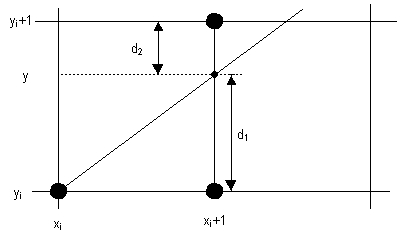
To summarise: Bresenham's algorithm at each step must make a decision between plotting (xk+1, yk) or (xk+1,yk+1), given that the ideal point to plot would be (xk+1, m*(xk+1)+b). To make this decision, we calculate the error rate of both choices, which we can define as their distance to the ideal point. As indicated in the figure we can then define:
Distance between "right-point" and "ideal point" = d1 = y
- yk
Distance between "right+above point" and "ideal point" = d2 = (yk+1) - y
We can then decide between these points by checking whether (d1 <= d2). If d1 <= d2 then we plot (xk+1,yk) during the next iteration, otherwise we plot (xk+1,yk+1). However, calculating these variables at each iteration is not going to result in an efficient algorithm. To speed things up, we introduce a "decision variable" which will be updated at each iteration. First of all, we rather test the sign of (d1-d2) rather than d1<=d2 because a comparison with 0 may be faster. Hence, if (d1-d2) > 0 choose (xk+1,yk+1), otherwise (xk+1,yk).
(d1-d2) = y - yk - ( (yk+1) - y) ) = y - yk - (yk + 1) + y.
Recall that y = (m*xk+1)+b, so by substitution:
(d1-d2) = m*(xk+1) + b - yk - (yk+1) + m*(xk+1) + b = 2m * (xk+1) - 2yk + 2b - 1.
Replacing m by dy/dx (with dy = |y2-y1| and dx = |x2-x1| ) we get:
(d1-d2) = 2*(dy/dx)*(xk+1) - 2yk + 2b-1 = 2*(dy/dx)*xk + 2*(dy/dx) - 2yk + 2b - 1.
This is a complex equation which we can simplify by multiplying both sides with dx. Multiplying by dx has no result on our test since dx is always positive, such that the sign of d1-d2 will not change.
Pk = dx*(d1-d2) = dx * ( 2*(dy/dx)*xk +
2*(dy/dx) - 2*yk + 2b - 1 )
= 2dy*xk + 2dy - 2dx*yk + 2dx*b - dx
= 2dy*xk - 2dx*yk + c (with c
= 2dy + dx(2b - 1) )
We now have our decision variable which can be calculated relatively efficiently. However, in its current form we still need to calculate it at each iteration. We can change this by only calculating the incremental differences between Pk and Pk+1. We can do so because changes in Pk are linear. So we calculate:
dP = Pk+1 - Pk
= 2dy*xk+1 - 2dx*yk+1 + c - 2dy*xk +
2dx*yk - c
= 2dy*xk+1 - 2dy*xk - 2dx*yk+1 +
2dx*yk
= 2dy*(xk+1 - xk) - 2dx*(yk+1 - yk)
= 2dy - 2dx(yk+1-yk)
Because we increase the x-value by 1 at each step, xk+1 - xk = 1. The value of (yk+1-yk) is less trivial, since it depends on the choice of the point. (yk+1-yk) = 0 if we choose (xk+1,yk), = 1 otherwise. So eventually, we get:
dP = 2dy - 2dx*(0) = 2dy when choosing the "right-point"
dP = 2dy - 2dx*(1) = 2dy - 2dx when choosing the "right+above point".
So now we know how to increase Pk to arrive at Pk+1 during each iteration. Such an addition is much more efficient than calculating Pk every time (cf. the DDA technique presented earlier). All that is left to define is the initial value of P, i.e. P0.
Pk = 2dy*xk - 2dx*yk + 2dy + dx(2b - 1)
P0 = 2dy*x0 - 2dx*y0 + 2dy + dx(2b - 1)
Since
b = y - mxk we get:
= 2dy*x0 - 2dx*y0 + 2dy + dx*(2*(y0 -
(dy/dx)*x0) - 1)
= 2dy*x0 - 2dx*y0 + 2dy + 2dx*(y0 -
(dy/dx)*x0) - dx
= 2dy*x0 - 2dx*y0 + 2dy + 2dx*y0 -
2dy*x0 - dx
P0 = 2dy - dx
We now have an initial test value for P. Depending on whether or not P is bigger than 0, we choose one of 2 points to plot during the next iteration. In addition, the test also determines how we have to update P for the next iteration. Given the above calculations, implement Bresenham's algorithm for lines in the first octant. When you got this working, extend your algorithm to work for arbitrary octants.