Introduction
Arbitrary curves are usually difficult to work with in computer graphics. An often used technique is to approximate the curve by means of many small line segments. The drawback of this technique is that you need a lot of lines to generate something that looks smooth enough to resemble the curve.
An alternative solution is to approximate the curve not by means of line segments but by means of polynomials of degree 3 (i.e. functions of the form f(x) = a0 + a1*x + a2*x^2 + a3*x^3). Usually, these are expressed in parametric form:

Parametric equations allow us to express the fact that there can be multiple y-values for a single x-value.
Source code for this session.
Exercises
Exercise 1: Bezier curves and de-Casteljau's algorithm
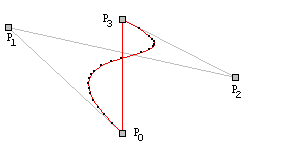
A Bezier curve is defined in terms of a number of control points. For example, a cubic Bezier curve is defined in terms of 4 control points P0, P1, P2, P3. To get an idea of the influence of a control point on the Bezier curve, you can experiment with the following Java applet:
 |
Applet source. |
P0 and P3 define the start and endpoints of the curve. P1 and P2 determine the initial direction of the curve. Hence, the curve is determined by 2 endpoints and the slope of two line segments (P1 - P0 and P2 - P3).
The parametric formula for the Bezier curve given 4 control points is the following:
PB = (1-t)3 P1 + 3t(1-t)2 P2 + 3t2(1-t) P3 + t3 P4
with 0<= t <=1
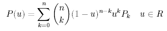
In the general case, for n control points, the following applies (u = t):
Alternatively, we can construct the curve by means of a recursive formula. This formula is due to Paul de Casteljau, which is why it's called de Casteljau's algorithm. It is based on the following recurrence relation:
![]()
The following applet demonstrates the algorithm:
For a fixed value of t, the approximation (the black dot) looks as follows:
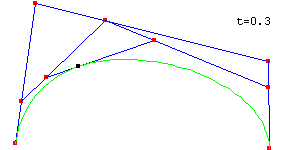
While the algorithm is slower than directly using the parametric formula, it is numerically more stable. Implement de Casteljau's algorithm for rendering (cubic) Bezier curves.
Exercise 2: Uniform B-Splines
B-splines are a generalisation of Bezier-curves. Given a set of n control points, a B-spline will approximate the curve piece-wise by means of a number of Bezier-curves.
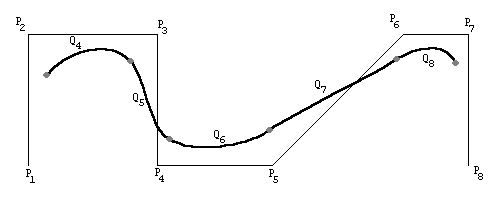
Let's say we have m control points: P0, P1,..., Pm. If we want to approximate the curve defined by these control points by means of cubic (3rd degree) Bezier curves, we will generate a number of curves Q3,Q4,...Qm (i.e. # curve segments = # control points - 3). Each curve segment Qi is defined by the control points Pi-3,Pi-2,Pi-1 and Pi. E.g. Q4 is a Bezier curve defined by P1,P2,P3,P4, Q5 is defined by P2,P3,P4,P5 and so on.
The mathematical formula for a curve given 4 control points (with 0 < t < 1) is:
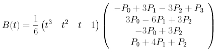
The advantages of using a B-spline rather than one big Bezier curve is that a B-spline is smoother at join points and requires less computation when a single control point is moved. A Bezier curve would have to be recalculated completely, while with the B-spline, only the 4 curves that depend on the control point need to be recalculated.
Implement a uniform B-spline approximation of a curve for an arbitrary number of control points based on the above formula.
PS. Non-uniform B-splines are splines in which the continuity of the curve can be broken at a control point.