Introduction
In this session, we will use an industrial-strength graphics library, to wit OpenGL. In previous sessions, we have implemented many low-level operations (drawing lines, clipping, projection) ourselves. However, these are tasks that are usually implemented by a graphics library like OpenGL. In this session, we will see how such libraries are used in practice.
OpenGL is a low-level graphics library specification. The library provides the programmer with a set of geometric primitives to e.g. render points, lines and polygons, to draw textures and to deal with lighting. Geometric figures can be rendered both in 2D as well as in 3D. OpenGL was originally developed by Silicon Graphics and is platform-independent. Usually, however, OpenGL is used together with a platform-dependent "binding" library that connects OpenGL to the underlying windowing system (e.g. Windows, X, Mac OS X).
The OpenGL API has originally been developed for C and C++, although there exist many bindings for other languages. In this session, we will make use of Processing's built-in support for OpenGL. The key functions that you need can be found in the extended API reference (especially under the headings "3D primitives" and "Transform").
All code for this exercise session.
Keep in mind that this lesson is only meant to serve as a "teaser" to get acquainted with OpenGL. It is impossible to learn all of OpenGL in just 2 hours. If you are interested in using OpenGL yourself, there exist tons of tutorials on the web (Google them!). I will demonstrate the basics of OpenGL by means of the example in ex0demo.pde (based on the original here). The code itself also contains plenty of comments.
As always in Processing, rendering is performed in the draw method.
void draw() {
  background(0);
  resetMatrix();
The first line ensures that we render from an empty (in this case black) canvas. You will soon find out that rendering 3D figures in OpenGL is all about matrix-manipulation. There are two important matrices in OpenGL: the projection matrix, which controls the camera (or viewpoint) and the modelview matrix, which controls where objects will be rendered. Note the similarities here with our own little 3D engine from session 7. In Processing, the matrix that is manipulated by default is the modelview matrix. The function resetMatrix() resets this matrix to the identity matrix. By doing so, we can draw our 3D models assuming that (0,0,0) refers to the middle of the screen. The X-axis increases from right to left, the Y-axis from top to bottom and the Z-axis inward to outward.
The translate(x,y,z) function applies a translation to the modelview matrix. By doing so, all subsequent drawing operations will be translated according to the vector (x,y,z). Note that the translation is relative to the current modelview matrix, not relative to the origin (of course, in this example it is relative to the origin because we reset the modelview matrix first).
translate(-1.5f,0.0f,-6.0f);
The translation moves the "origin" from which to draw to the right of the screen, and also a bit deeper (-6.0 units). To actually plot a point, you use the vertex(x,y,z) function. Before you can start plotting, you have to tell OpenGL that it should interpret all subsequent calls to vertex as vertices of a triangle. This is done by a call to beginShape, which takes as argument the type of figure to plot (in this case TRIANGLES). See the reference of the beginShape function for other possible options. The figure below illustrates some of them as well:
We will only plot one triangle, so we make just 3 calls to vertex. However, if we would have liked to draw 2 triangles, we could have just made 6 calls to vertex, and OpenGL would know that the 6 vertices define 2 triangles, because of the TRIANGLES option. We can colour the triangle by assiging a fill color to each of the vertices.
beginShape(TRIANGLES); // tell OpenGL that the following vertices define a triangle
  fill(1.0f,0.0f,0.0f); // color = red
  vertex( 0.0f, 1.0f, 0.0f); // top vertex
  fill(0.0f,1.0f,0.0f); // color = green
  vertex(-1.0f,-1.0f, 0.0f); // lower right
  fill(0.0f,0.0f,1.0f); // color = blue
  vertex( 1.0f,-1.0f, 0.0f); // lower left
endShape();
The triangle is drawn on the right-hand side of the screen. Now, we will plot a square to the left of it. To move towards the left, we translate again, this time 3 units to the left (1.5 units back to the center, then another 1.5 units towards the left).
translate(3.0f,0.0f,0.0f);
To plot the square, we use the QUADS option, causing OpenGL to automatically interpret 4 subsequent calls to vertex as the vertices of a quadrilateral (a four-sided polygon). Note that the vertices are drawn in clockwise order: top left, top right, bottom right, bottom left. In OpenGL, polygons whose vertices are specified clockwise face away from the front view (which means you will see their back), while polygons whose vertices are specified counter-clockwise face the front view.
    beginShape(QUADS); // Draw quadrilaterals (i.e. 4-sided polygons)
      vertex(-1.0f, 1.0f, 0.0f); // Top Right
      vertex( 1.0f, 1.0f, 0.0f); // Top Left
      vertex( 1.0f,-1.0f, 0.0f); // Bottom Left
      vertex(-1.0f,-1.0f, 0.0f); // Bottom Right
    endShape(); // Done with the square
Exercises
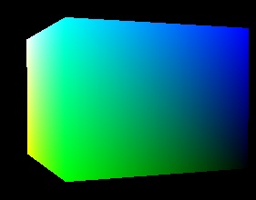
Exercise 1: Spinning Cube
This program renders a 3D cube, then continuously rotates the camera around the cube. Have a look at the source code and try to understand what is going on. Try to play with the different parameters to find out what their effect is.
Use the translate(x,y,z) function to let the cube move clockwise or counterclockwise around the screen. For this, you will need to add some additional "motion variables" that have to be updated on each drawing step. Note: only manipulate the modelview matrix after all calls to camera and perspective have been made (otherwise, Processing seems to disregard their effects).
Next, try to shrink and grow the cube between a certain minimum and maximum-value such that it appears as if the cube is bouncing. This can be done by means of the scale(x,y,z) function.
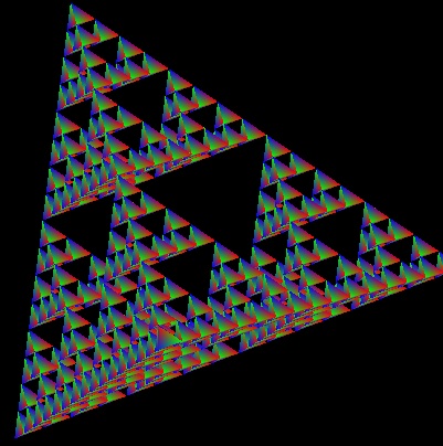
Exercise 2: 3D Sierpinski Triangle
Do you recall the Sierpinski triangle from Session 4? In this exercise, we will plot the fractal in 3D rather than in 2D. To do so, you have to plot smaller triangles that recursively form bigger triangles. The code contains a recursive function to draw the triangle. In each call (other than the base-case), you need to construct 4 sub-tetrahedrons by recursively calling the function four times. However, in each call, the 4 sub-tetrahedrons should be:
- scaled 50% smaller
- translated such that 3 of the 4 smaller pyramids are placed next to each other, and the fourth one is put on top of these 3
Nno parameters are passed to the recursive function to keep track of the scaling and the translation. Instead, use the implicit modelview matrix for this. You will need to "undo" the modifications the call has made to the modelview matrix when the recursive call returns. To "save" and "restore" the state of your modelview matrix, use the pushMatrix() and popMatrix() functions. The user can himself define the recursion depth by means of the '+' and '-' keys, and can rotate the sierpinski triangle by means of the arrow keys.
In this exercise session, we have only uncovered the basics of OpenGL programming. There are more advanced aspects, such as texture mapping and lighting which we will not discuss here. However, you can learn a lot from the examples on the Processing website. For those interested, the above exercises are also available in C here.